Incidental ingestion of soil is thought to result primarily from hand-to-mouth activities transferring soil adhering to skin. Thus, for human health risk assessment, the soil bioavailability of greatest interest is that associated with soil particles in size ranges most likely to adhere to skin. Soil bioavailability studies have used soils sieved to various size ranges. Perhaps the closest value to a standard size emerged from soil bioavailability studies for lead and arsenic in the 1990s, which typically used soil sieved to <250 µm (Ruby and Lowney 2012). USEPA recommended that the <250 µm size for measuring soil lead concentrations be used in the IEUBK model (USEPA 2000a). The rationale typically given for this value is that it encompassed the particles most likely to adhere to a child’s hands. However, more recent soil adherence studies suggest that a particle size limit of <150 µm better reflects the soil particles that would adhere to hands under most conditions (Ruby and Lowney 2012). The USEPA now recommends that soil used for lead bioavailability studies should be sieved to < 150 µm (USEPA 2016e). Although this guidance is for lead bioavailability studies, the same recommendation logically applies to bioavailability studies with other contaminants. Further, the issue of appropriate soil particle size for study applies not only to animal studies, but human and in vitro studies as well.

For risk assessment purposes, the most relevant bioavailability information is the relative bioavailability of the chemical from soil. This value indicates how the bioavailability of the chemical from soil compares with its bioavailability implicit in the toxicity value (for example, oral reference dose or cancer slope factor) used to estimate risk (NRC 2003; USEPA 2007c). The bioavailability implicit in the toxicity value is the bioavailability that occurred when the chemical was administered in the critical study on which the toxicity value is based, such as from food, water, or oral dose vehicle. Thus, to develop a relative bioavailability estimate, the study should include a comparison group dosed as near as possible to animals in the critical toxicity study, minimally, with the same dosing medium (food, water, or oral dose vehicle).

A variety of endpoints can be used to attempt to measure the systemically absorbed dose of a chemical. To develop quantitative bioavailability values, whatever is being measured must consistently reflect this dose. For example, if a tissue concentration is being used to measure the systemically absorbed dose, then the concentration should double when the systemically absorbed dose doubles, and decrease by 30% when the systemically absorbed dose decreases by 30%. The condition under which this consistent relationship is observed is termed linear pharmacokinetics (Shargel and Yu 1999). Although the processes determining the pharmacokinetics of a chemical are typically nonlinear, within a relevant range of doses and exposure conditions they are often sufficiently linear that linearity can be assumed. If conditions of the study cause this relationship to change and nonlinear pharmacokinetics occur, then errors in bioavailability estimates can result.

Nonlinearity typically occurs when the doses extend into a range where saturable or capacity-limited uptake or metabolic processes occur (Shargel and Yu 1999). A bioavailability study must demonstrate, or have good reason to assume, that the doses being used result in linear pharmacokinetics, or that RBA is calculated using appropriate nonlinear models that relate absorbed dose to external dose. For example, in the swine assay, RBA is calculated from blood lead area under the curve (AUC) using a regression model of the nonlinear relationship between dose and AUC.

Repeated doses resemble the conditions under which most environmental exposures occur and, for chemicals that bioaccumulate, can result in higher concentrations in blood, urine, and tissues that are easier to measure. When repeated doses are used, concentrations should be allowed to reach steady-state if possible. Steady-state conditions are reached when blood and tissue concentrations plateau. The time to reach steady-state depends upon the elimination rate of the chemical and can vary from hours to years.

If repeated doses produce a change in the rate of elimination of the chemical, for example, from metabolic enzyme induction (metabolic clearance), then determining relative bioavailability becomes complex. A change in metabolic clearance changes the relationship between the systemically absorbed dose and bioavailability endpoints such as blood, tissue, and urine concentrations. For example, an increased rate of metabolic clearance from induction (adaptive increase in the metabolism of a chemical) after several doses can lower blood concentrations, even if the bioavailability is unchanged. This situation is analogous to the problem that occurs with nonlinear pharmacokinetics, in which the consistent relationship between systemically absorbed dose and the endpoint being measured is lost. For valid comparisons among treatment groups to be used to estimate relative bioavailability, the metabolic clearance of the chemical should be the same for each of the groups.

Dose-related enzyme induction complicates the comparisons between treatment groups. One way to avoid this problem is to evaluate bioavailability after a single dose. Metabolic clearance should be similar among naïve (previously untreated) animals given a single dose, allowing more straightforward comparisons among treatment groups. This approach addresses the goal of determining the influence of a soil matrix on delivery of a systemically absorbed dose (the RBA) without the confounding influence of downstream events such as changing metabolic clearance.

Often, a chemical must be measured in its various forms (parent and metabolites) in blood, tissues, or urine to ensure that all the systemically absorbed dose is accounted for. From an analytical standpoint, this measurement is relatively straightforward for inorganic compounds. For example, arsenic bioavailability from soil in vivo is typically determined from total excretion of arsenic in urine. For organic compounds, however, the study must be conducted with a radiolabeled compound or else quantifying all metabolites can be challenging. Typically, the analysis focuses on the parent compound (if not extensively metabolized) or one or more major metabolites. Even though this approach does not capture all the systemically absorbed chemical, valid comparisons among groups to determine relative bioavailability can be made if it can be assumed that the analytes comprise a consistent percentage of the total chemical present (parent plus metabolites). This assumption is usually reasonable if the doses are in the linear pharmacokinetic range and enzyme induction or some other change in metabolic clearance is not in play.

Metabolism of the chemical may be different in the animal model than in humans, and consequently the metabolite to be measured to capture most of the absorbed dose may be different from what would be selected if the study were conducted in humans. If differences in metabolism are recognized and taken into consideration, then they do not compromise the animal model, because the focus of bioavailability studies is on relative absorption rather than metabolism.

Determining an adequate number of subjects is based upon two opposing considerations: (1) a desire to have enough statistical power to detect differences among treatment groups; and (2) the cost of the subjects. Typical group sizes for primate studies are three to five animals per group (for example, Freeman et al. 1995; Roberts et al. 2002), while studies with less expensive animals (swine, laboratory rodents) generally use group sizes of six to ten animals per dose group (for example, Brattin and Casteel 2013; Bradham et al. 2013).

The number of animals included in each dose group may be used to inform the study design. For example, use of a crossover study design, in which each animal is used to generate data for both the soil dose and the reference dose, can increase statistical power compared to dosing separate soil and reference groups of animals. This practice assumes adequate depuration (elimination from the body) between trials and that considerations such as enzyme induction are not involved, which can occur especially with organics. Therefore, crossover studies should demonstrate that enzyme induction (if relevant) and depuration have returned to baseline state between dosing with site and reference soils.

Testing a range of doses helps to establish that pharmacokinetics are linear over the dose range to be studied. This testing also can be used to determine whether bioavailability depends on the concentration of the chemical in soil. One key issue common to in vivo studies is a limited ability to evaluate bioavailability at the lower end of the range of environmentally relevant doses. This problem is related to analytical sensitivity in measuring the chemical or metabolites in biological media, or in some cases, difficulty in distinguishing low doses from background exposures. Although the lower limit of soil concentration at which relative bioavailability can be reliably measured varies by chemical (and to some extent by the in vivo model system used), the lower limit can be substantially above the concentrations at which risk-based decisions must be made. Using these data requires the assumption that bioavailability data obtained for high soil concentrations applies also at lower concentrations, which may or may not be the case.

The study method should provide reliable data across the full range of RBA values that would be expected to exist at contaminated sites. This ability may be demonstrated through the study of a variety of test substrates. If the test substrates do not yield a wide range of values, then appropriate control samples may be developed to provide data across the desired range. Note that this point relates to variability in RBA contributed by physico-chemical interactions between the contaminant and soil, but does not address the range of RBA values that might exist among exposed individuals due to physiological and other variables. Examples of variables that could lead to interindividual RBA differences include age, presence and type of food in the GI tract, pregnancy, use of medications that affect GI function, and the presence of acute or chronic diseases. The individual variability in RBA that exists among humans exposed to the same contaminated soil is not well quantified in any current RBA experimental design.

One experimental design involves administering both a dose in soil and another comparison dose (such as in food or water, as appropriate) on separate occasions to each subject so that individual RBA values can be calculated. RBA results for each test soil sample are expressed as the mean ± standard deviation or standard error for results from the individual subjects. This design has been applied principally in studies using primates or humans. Studies in other species typically divide subjects into two or more groups, with some subjects receiving the chemical in soil and others receiving the comparison dose. No subject receives both doses, and RBAs for test soil samples in individual subjects consequently are not derived. Results from the soil and comparison groups are compared and RBA results are expressed as an estimate of the mean with confidence intervals for each test soil. Either design may be adequate for risk assessment, depending upon the objectives, but note that these two designs provide somewhat different information about the RBA of a given soil sample and require different statistical approaches.

Mass balance is an accounting of the fate of the contaminant through measurement of the disposition of the administered dose—how much was absorbed and excreted, how much was not absorbed, and how much remains in the body. Although not an absolute requirement, accounting for most or all of an administered dose in a bioavailability study helps to reduce any concerns that the absorbed dose may have been under- or overestimated.

Concentrations of parent chemical, metabolites, or both are measured in whole blood, or more commonly, serum or plasma. By taking blood samples over time, a concentration versus time profile can be generated from which the area under the curve (AUC) can be calculated. The AUC is expressed as the integration of chemical concentration in blood over time (for example, µg-hr/L), and provides a measure of the systemically absorbed dose. When compared against AUC for an intravenous dose, this method is the classical approach for determining bioavailability. The timing of blood samples should allow for adequate characterization of the increase, peak, and decline in concentrations over time. Too few time points or too few time points with measured concentrations result in a poor estimate of the AUC and substantial error in the calculated systemically absorbed dose. Bioavailability studies should show at least example blood concentration versus time curves to demonstrate adequate characterization of the AUC, especially at the lowest doses.

RBAs are calculated from AUC data using the following formula:

where the comparison dose is given in food, water, oral dose vehicle, or other medium as appropriate (see Relevant Comparison Group). If the dose from soil and the comparison dose are equivalent, then these terms cancel and the RBA is simply the ratio of the AUCs from soil and the comparison group. If the doses are not equal, then the AUCs can be corrected, as in the formula above. This correction can only be made, however, if the doses are in the linear pharmacokinetic range. Figure 5-1 shows as an example a comparison of blood concentration versus time profiles for benzo(a)pyrene (BaP), given in the same dose in food versus in soil from three difference sources (solvent, soot, and fuel oil). These blood concentration curves, and the AUCs derived from them, show reduced benzo(a)pyrene from soil regardless the benzo(a)pyrene source.

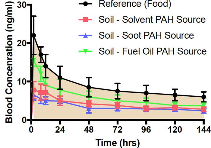
Figure 5‑1. Blood concentrations over time following oral administration of benzo(a)pyrene(BaP) in food or weathered soil in rats.
Source: Figure derived from data published in (Roberts et al. 2016).

The black reference line is the blood concentration over time of benzo(a)pyrene (BaP) and metabolites following administration of a single dose of BaP in food by oral dose vehicle. Blue, red, and green profiles are for the same dose of BaP from weathered soils with solvent, soot, or fuel oil as the BaP source. BaP concentration in food and soil samples was 10 ppm. Results are expressed as mean ± standard error of the mean (SEM), N=5 (Roberts et al. 2016).

Occasionally, attempts are made to estimate bioavailability from a blood concentration taken from a single time point. This approach assumes that the shape of the blood concentration over time profile is the same regardless the dosing medium, and that the ratio of blood concentrations at a given time point for soil and for comparison doses accurately reflects the ratio of their respective AUCs. Often, however, the shape of the blood concentration versus time profile changes when a chemical is given orally in different media, even when the total dose that is systemically absorbed over time is the same. For example, the rate of absorption from different dosing media might vary, causing the peak blood concentration to occur at a different time. The ratios of blood concentrations at most individual time points then can have little or no relationship to the ratio of the AUCs. Consequently, this approach is not recommended unless the pharmacokinetics of the chemical from the relevant oral dosing media are the same as the pharmacokinetics from soil, the pharmacokinetics are well characterized in the animal model (which is seldom the case), or the chemical has been dosed repeatedly and the blood concentrations are at steady-state.

Figure 5-2 shows hypothetical blood concentration versus time profiles for the same chemical from two different environmental matrices. The blue curve shows that absorption was rapid from the environmental matrix, while the red curve shows that release and absorption occurred more slowly. The slower release and absorption results in lower concentrations at earlier time points but somewhat higher concentrations at later time points. The extent of absorption—the bioavailability—is the same from both matrices, and both profiles have the same AUC. If bioavailability had been determined by measuring blood concentrations at a single time point, then a sample taken less than 12 hours after the dose could have led to the erroneous conclusion that bioavailability was substantially greater for the blue line conditions. Similarly, a sample taken after 24 hours might lead to the erroneous conclusion that bioavailability was somewhat greater for the red line conditions.

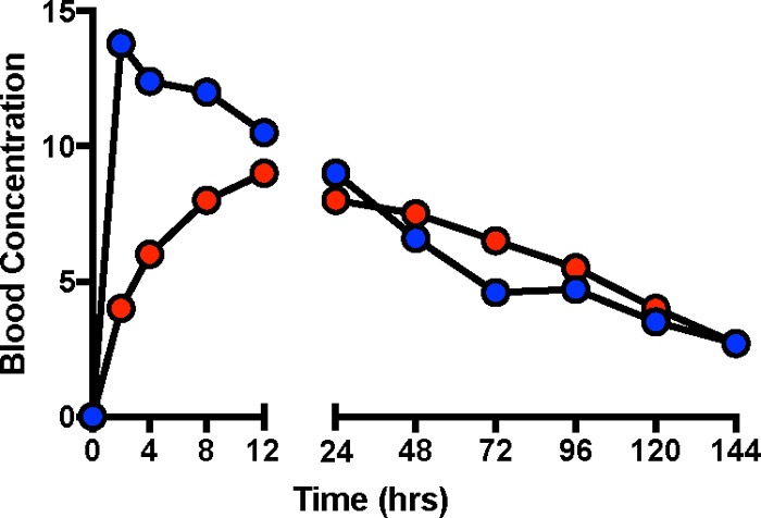
Figure 5‑2. Different blood concentration profiles despite the same bioavailability.

Figure 5-2 shows hypothetical blood concentrations curves for the same chemical ingested in two different matrices (such as food and soil), with initial absorption more rapid from one of them. In this example, although the blood concentration curves over time differ, the absorbed dose is the same—the curves have the same AUC. This example illustrates the problem of comparing absorbed doses under two sets of conditions by looking at blood concentrations at a single time.

A chemical can only appear in urine after systemic absorption, and urinary excretion is a common measurement endpoint for bioavailability assessment. This approach works best when urinary excretion is the major pathway of elimination and occurs over a time frame in which elimination of most of the administered dose can be captured. Measurement can be focused on parent chemical plus metabolites, as is common in bioavailability studies for inorganics such as lead and arsenic, where total urinary excretion of the element is measured. Measurement can also be focused on the parent chemical alone (if a large fraction of the chemical excreted unchanged in urine) or metabolites alone (if metabolism is extensive, usually limited to one or a few major metabolites). Urine is usually collected over one to several days, depending upon the rate of urinary excretion, and the total mass appearing in urine is compared with the administered dose to estimate the bioavailability:

Where: U is the total mass excreted in urine

As with blood data, urinary excretion can be corrected if different doses are used in the soil and comparison groups, but only if the pharmacokinetics are assumed or shown to be linear.

Excretion of chemical in the feces can also be used to estimate the systemically absorbed dose if the mass excreted in feces can be assumed to represent unabsorbed dose from the gastrointestinal tract. Biliary excretion confounds this approach by reintroducing absorbed chemical, usually in the form of metabolites, into the gut where it can be eliminated in feces along with unabsorbed material. Microbial metabolism of the chemical within the GI tract can also be a confounding influence, complicating quantification of what exactly represents absorbed versus unabsorbed chemical. This approach works best when biliary excretion of the chemical is negligible and microbial metabolism is limited.

Experiments in which excreta are used as endpoints are conducted in metabolism cages to facilitate the separation and collection of urine and feces. Collection surfaces within the cages are usually plastic, glass, or Teflon. The choice of material can be an important consideration, because some chemicals or metabolites stick to certain surfaces (for example, PAH metabolites to plastic), resulting in incomplete recovery. Cage designs also vary in the efficiency with which feces and urine are separated. No design is perfect, and some degree of cross-contamination is expected. This contamination poses a problem when the excreta that is not the measurement endpoint has enough of the chemical or metabolites present to cause significant contamination. An example of this effect is presented in the PAHs chapter, where the small mass of metabolites present in urine may be significantly affected by even small contributions from fecal contamination.

Tissue concentration measurements can also provide an indication of the systemically absorbed dose, and thus be used to determine RBA. Using tissue concentrations as a measurement endpoint can be advantageous if there are problems with blood or excreta approaches, such as when blood concentrations are low or taking repeated blood samples is impractical, metabolism cages for collection of excreta are unavailable, or metabolism or excretion pathways of the chemical prevent using urinary or fecal excretion as the measurement endpoint. Generally, tissue concentrations are measured once after the experimental animal has been euthanized. The same problem with measurement of the concentration in blood at a single time point exists for tissues—a difference in the concentration profile over time when a single dose is administered in different media can produce errors in comparison of the systemically absorbed dose. Consequently, tissue concentration measurements are best determined after repeated dosing to steady-state. The use of repeated doses creates a difficult situation if the clearance of the chemical changes, such as with induction of metabolism (see Repeated versus Single Dose).

Although not commonly used, biomarkers have been proposed as measurement endpoints for determination of the bioavailability of contaminants from soil, notably with PAHs. A brief discussion of the rationale and limitations of these endpoints is presented in PAHs chapter.